[AI Inspection: Challenges in the Field (1)] Starting AI Inspection Without Defective Products

In inspection automation meetings with manufacturing customers, the first thing we check is how many defective samples they actually have.

The answer is almost always the same: five or six samples for one defect type, one sample for another, and sometimes none at all if it is a newly launched production line.

From a manufacturing perspective, this is a good situation—it means the process has a high yield. From a training-data perspective, however, it is a problem. And this is not simply a matter of “collecting more data” by investing more time. Even once data starts to accumulate, the problem does not end. Instead, other challenges begin to emerge.

After more than 100 PoCs and over 30 production deployments, we repeatedly encountered bottlenecks at the same points and found that these challenges were closely interconnected. This article summarizes the five key challenges we identified. We will cover how we addressed each of them in the following articles.

1. Defect Data Accumulates Slowly

The defect rate on a stable production line is typically below 1%. Even when tens of thousands of units are produced every day, a specific defect type may occur only once a month, if at all.

Collecting enough samples for model training can therefore take weeks or even months. During that time, additional effort is required to store, capture, and label each sample.

For a new production line or a new product, the starting point may be zero defect samples. In practice, this waiting period alone can prevent an AI inspection project from getting off the ground. In many cases, the project is stalled not because the technology is lacking, but because there is simply no data to start with.

That does not mean we can intentionally create defects by running the production line under abnormal conditions. Artificially induced defects often differ in shape from naturally occurring defects because their underlying mechanisms are different. Ultimately, we have to wait for defects to occur naturally.

2. Defect Samples Are Unevenly Distributed Across Types

Even after collecting data, samples do not accumulate evenly across defect types. Two or three frequently occurring defects tend to account for most of the data, while dozens of other defect types may have only one or two samples each.

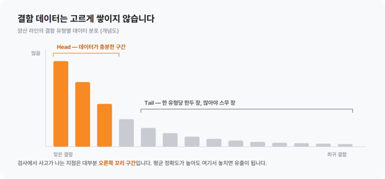
[Figure 1] Distribution of Samples Across Defect Types

A model’s average performance is largely determined by the high-volume portion of the dataset. However, actual inspection escapes often occur in the long tail.

This is why a detection rate of 98% is not necessarily reassuring. The remaining 2% can mean something completely different depending on which defect types they represent.

A common response is to oversample rare classes. But when there are only one or two original samples, this comes close to showing the model the same images repeatedly. Even with rotation, flipping, or brightness augmentation, the diversity of the actual defect patterns does not increase.

On a real production line, defects of the same type can vary in orientation, depth, and length from one occurrence to another. No amount of augmentation applied to two original images can recreate that real-world variation. The result is often greater overfitting rather than better generalization.

3. Labeling Errors Are Mixed into the Training Data

Training-data labels are created by people. Inspection criteria can vary slightly from one inspector to another, and samples near the pass/fail boundary can receive different judgments even from the same inspector on different days. Data-entry errors can also occur during shift changes.

In some projects, we found that 30–40% of the training data we received was contaminated. Here, “contaminated” refers to cases where defective samples were included among images labeled as good, or where the wrong defect type was assigned.

When defective samples are placed in the good-product folder, the model learns those defects as part of the normal range. As more data is added, the decision boundary can actually become less clear rather than more accurate.

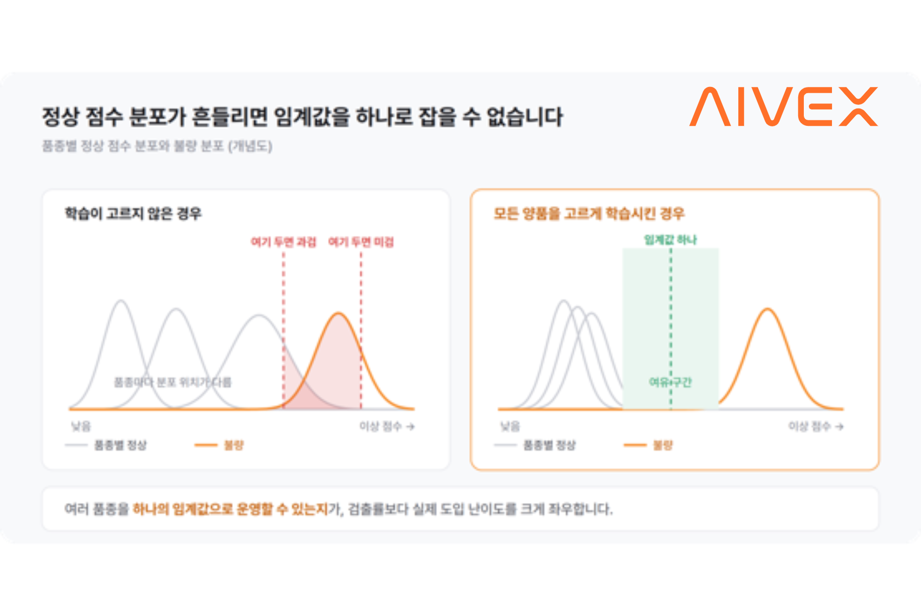
This problem is difficult to detect. If the validation set has been labeled by the same people using the same criteria, the metrics may look perfectly normal. In fact, the model may appear even more accurate because it has learned the inspectors’ labeling errors as well. The mismatch only becomes apparent after deployment on the production line.

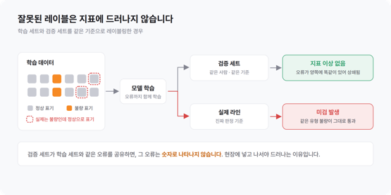
[Figure 2] When the Training and Validation Sets Share the Same Labeling Errors

Managing borderline samples separately can mitigate this to some extent. Having multiple inspectors independently evaluate the same samples can reveal disagreements before the data is used for training.

However, this requires additional operational effort, and collecting such samples while a production line is running is not always easy.

4. Defects That Were Not Present in the Training Data Eventually Appear

As process conditions change, raw-material lots are replaced, and equipment ages, new defect patterns that were not present during training inevitably emerge.

This is not a question of possibility—it is a matter of time.

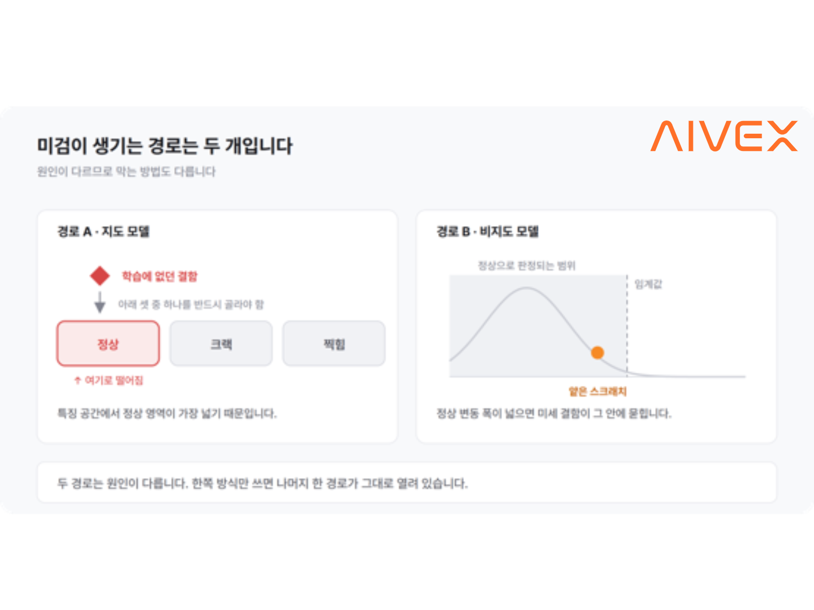
A classification model has to assign every input to one of the classes it learned. When it encounters an unfamiliar pattern, it has no option to say, “I don’t know.” Instead, it assigns the input to the class that appears most similar, which is often the normal class.

The problem is not simply a slight drop in performance. Defective products can pass through inspection and move on to downstream processes.

A common approach is to filter inputs using softmax confidence scores. However, this is difficult to rely on because models can still produce high confidence for inputs they have never seen during training.

The model does not know what it does not know.

5. The Number of Models Grows with the Number of Product Variants

When a separate model is built for each product variant, 200 product variants mean 200 models.

That also means 200 training datasets, 200 monitoring targets, and 200 rounds of retraining, validation, and deployment whenever process conditions change.

When a new product variant is introduced, data collection has to start again from scratch. This can take several weeks for a single variant.

Once the number of product variants reaches the thousands, this approach breaks down—not because of model performance, but because of operational complexity.

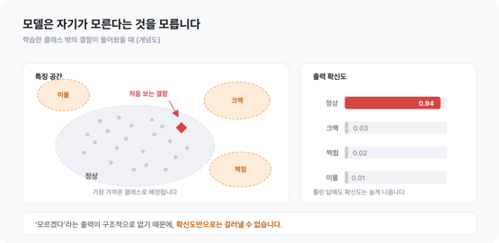
[Figure 3] How Inputs Outside the Trained Classes Are Handled

Summary

The five challenges above have one thing in common: they are fundamentally data problems, not model problems.

Replacing the backbone with a newer architecture or increasing the number of parameters does not make these problems go away.

Based on this, we took four directions:

• Train directly on raw data containing noise and long-tail distributions, rather than assuming the data can be perfectly cleaned beforehand.

• Use both supervised and unsupervised learning tracks so that unseen defects are not simply classified as normal.

• Generate additional samples when real defect data is insufficient.

• Keep a single model even as the number of product variants grows.

There is one more challenge.

Even if all four of the above problems are solved, performance will still suffer if the imaging conditions vary from one inspection to another. On a multi-product production line, manually aligning the optical system for each product variant creates an operational burden that grows on the same scale as the problems described above.

In the following articles, we will address these challenges in order:

Part 2. What Actually Goes Wrong When Detecting Anomalies Using Only Normal Samples
Part 3. Why AIVEX Combines Supervised and Unsupervised Learning in a Single Model
Part 4. How We Processed Thousands of Product Variants with a Single Model
Part 5. What to Consider When Generating Defect Data for Model Training
Part 6. The Problem of Manually Aligning the Optical System Whenever the Product Variant Changes