[AI Inspection: Challenges in the Field (3)] Why AIVEX Combines Supervised and Unsupervised Learning in a Single System

At the end of Part 2, we left one limitation of the unsupervised model on the table: it only tells you whether something is anomalous, not what kind of defect it is. But the field needs the kind. Defect-type trends are what drive process improvement, and whether a part gets reworked or scrapped depends on the type.

Yet relying on supervised learning alone brings back the fourth problem from Part 1: the model classifies defects it never learned as normal. Instead of picking one of the two, we decided to put both approaches into a single system — and this post is about that architecture.

There are two paths to a miss

Let's settle the premise first. In inspection, what turns into an incident is not overkill but the miss. Overkill gets filtered out downstream when a person takes a second look; a miss ships as-is.

But a miss doesn't arise through just one path. There are two, and their causes differ.

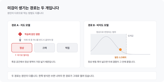
[Figure 1] How misses arise in each approach

Path A comes from the supervised model. A classifier must pick one of the classes it was trained on. When a never-before-seen pattern comes in, there is no output that means "I don't know," so the classifier assigns the input to the nearest class in feature space. And the normal class, having the most training data, occupies the widest region of that space. As a result, a large share of unknown defects lands in normal.

Here the question naturally comes up: "Then why not add an unknown class and train on it?" To do that, you would need training data for unknown — and if you already had that data, it wouldn't be unknown in the first place. Adding classes cannot close this problem.

Path B comes from the unsupervised model. Widen the normal range to reduce overkill, and shallow scratches or small foreign particles slip inside it. This shows up especially often on products with complex background patterns. It is also where the score-distribution problem from Part 2 carries straight through.

The two paths have different causes, so blocking them requires different means. Use only one approach, and the other path stays open.

We run the two models independently

The configuration is simple. The same image goes into a supervised model and an unsupervised anomaly detection model separately, and the two outputs are merged afterward.

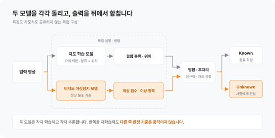
[Figure 2] Running the two models independently and merging their outputs

The supervised model outputs learned defects with their type and location. The unsupervised model outputs the degree of deviation from the normal distribution and the anomalous region. The two models share no features and no weights — each trains on its own, each infers on its own. Because the overall configuration handles inputs beyond the trained class set, it falls under what is called Open-set Recognition.

The reason we keep the two models apart is that their training cycles differ. The supervised model must be retrained whenever new defect samples accumulate; the unsupervised model is updated when the good-part data changes or process conditions shift. Couple them into one, and a single retraining moves both decision criteria at once. You add one new defect to the supervised model, and suddenly the unsupervised threshold has to be re-tuned — and the entire line has to be re-validated every time.

The independent configuration has a cost: each image requires two inference passes. Since the judgment must finish within the line's takt time, the two models run in parallel rather than sequentially — and this is where the inference optimization covered in Part 4 becomes necessary. We accept this cost in exchange for simpler operation.

Aligning formats before merging

Merging is done at the region level, not the image level. A single image can contain multiple defects, some of which are known and some seen for the first time. Attach one judgment per image, and that distinction disappears.

But since the two models are independent, their output formats differ. They cannot be overlaid as-is, so two things are aligned first.

One is the scale. The supervised model outputs defect regions as masks, while what the unsupervised model produces is a continuous-valued map holding a deviation score per pixel. Turning that map into regions requires binarization — deciding above which value counts as anomalous — and that criterion is drawn from the score distribution of normal data. The score-distribution stability from Part 2 becomes necessary again here. If the unsupervised model's score distributions sit at different positions per variant, the binarization criterion also varies per variant, and no single merging rule can be established.

The other is the coordinate system. The two models output at different resolutions. The unsupervised anomaly map typically comes out at the backbone's feature-map resolution and is upscaled to the input size, while the supervised segmentation comes out at the input resolution. Boundaries smear during upscaling, so the two results must be resampled into the same coordinate system before their positions can be compared.

Measuring overlap and splitting into three cases

Once aligned, the regions produced by the two models are overlaid, and the degree of overlap is measured with IoU. The result falls into one of three cases.

If the overlap exceeds the criterion, the two models are taken to be pointing at the same defect, and the supervised model's judgment takes precedence in fixing the class — the unsupervised model can only say that something differs from normal, while the supervised model provides both the type and the boundary. However, even with overlap, if the supervised model's class confidence is low, the class is not fixed and the case is passed on as Unknown. When both models point at the same location but the type is uncertain, it may be something similar to a learned class yet different.

A region detected only by the unsupervised model is treated as Unknown and sent to a person. This is most likely a defect the supervised model has never learned — and this is the point where Path A gets blocked.

A region detected only by the supervised model stays as Known. This is the case where the unsupervised model absorbed the defect into normal variation; if it is a type the supervised model has already learned, that judgment is trusted. This is where Path B gets blocked.

The two miss paths correspond to the latter two cases, one each — cases that either model alone would have missed.

Unknowns become training data again

The practical benefit of this architecture reveals itself during operation.

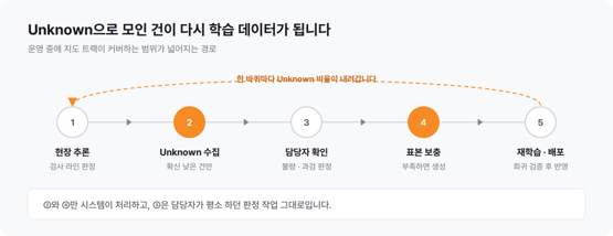
[Figure 3] How cases collected as Unknown flow back into training data

Samples the unsupervised model classifies as Unknown are automatically collected on the side. A quality staffer on the floor only needs to confirm whether each is a real defect or overkill, and that judgment becomes the material for the next round of training. When samples are scarce, the generation methods covered in Part 5 fill out the quantity before the samples are folded into the supervised track.

With each cycle, the range of defects the supervised model covers widens, and the unsupervised model's role narrows toward being a safety net for the regions not yet learned. The Unknown rate comes down naturally.

No AI engineer needs to be stationed on-site for this. The judgment work the staffer was already doing becomes the training input as-is. Retrained models, however, are not deployed straightaway: a newly folded-in class can degrade performance on existing classes, so the update goes live only after regression validation confirms that no item has dropped below the previous version.

Where this architecture breaks down

The hybrid is not always a win. If the unsupervised model's binarization criterion is not properly set, the detected regions themselves become unstable and the merging rules lose their meaning. Set the criterion too high, and the unsupervised side produces no regions at all — the system effectively degenerates into supervised-only. Set it too low, and most of the frame gets flagged as anomalous, and nearly every case gets passed on as Unknown.

So we sequence deployment like this. Early in a line's life, we start with unsupervised only — there is no defect data, so the supervised model has nothing to learn. During this period, the normal score distribution is stabilized on good-part data, and once defect samples accumulate through Unknown review, the supervised model is attached. Reverse the order, and the merge never holds.

On thresholds

To the question "is a bit more overkill acceptable?", the answer differs line by line. But the principle we hold to is a single one: block misses with architecture; regulate overkill with thresholds and downstream review.

A miss is a problem of closing an open path, so lowering thresholds does not solve it. A defect the model never learned remains, no matter how low the threshold goes, closest to normal inside the classifier. Overkill, by contrast, is a problem thresholds and review procedures can handle. This is why the two tracks are used together — each of the two miss paths described above is blocked by a different track.

In the next post, we cover what it takes to scale this architecture to thousands of product variants.

[AI Inspection: Challenges in the Field] Series

Part 1. Starting AI Inspection Without Defective Products
Part 2. What Actually Goes Wrong When Detecting Anomalies Using Only Normal Samples
Part 4. How We Processed Thousands of Product Variants with a Single Model
Part 5. What to Consider When Generating Defect Data for Model Training
Part 6. The Problem of Manually Aligning the Optical System Whenever the Product Variant Changes