[AI Inspection: Challenges in the Field (2)] Where Anomaly Detection Breaks When Trained Only on Normal Data

In Part 1, we laid out five points where inspection AI repeatedly gets stuck. This post takes on the first of them: starting AI inspection when you have no defect images to train on.

The idea behind unsupervised anomaly detection is simple. If you can't teach the model what defects look like, don't teach it defects at all. Instead, use only normal-data images to build a reference for "this is roughly what normal looks like," then score each incoming image by how far it deviates from that reference.

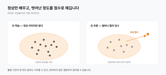
[Figure 1] Building a reference from normal data only, and converting deviation into a score

In practice, this approach offers three advantages. First, engineers can train a model without defining defect types in advance. Second, the model flags defects that were never on the inspection checklist. Third, normal images accumulate simply by running the line, so the approach can be deployed on new lines right away.

Up to this point, everything checks out on benchmarks. The problems begin when production data starts flowing in.

Start with how the anomaly score is computed

To explain where the unsupervised approach breaks down on a production line, we first need to look at how the model computes its anomaly score.

A widely used setup works like this. Normal images are passed through a pre-trained backbone to obtain feature maps from intermediate layers. Rather than compressing each feature map into a single vector per image, the map is split into patches, which are stored in a memory bank. At inference time, patches are extracted from the input image in the same way; each patch's distance to the stored normal patches is measured, and the largest of those distances becomes the image's anomaly score.

The model splits images into patches because defects are local. Compress an entire image into one vector, and a scratch covering 1% of the frame gets diluted by the 99% of normal pattern around it. Split the image into patches, and the score spikes only in the patches containing the defect, so the signal survives. As a bonus, knowing which patch scored high directly provides location information — the defect region comes out without attaching a separate detector.

Patch size is not a value an engineer can set arbitrarily. If the patch is much larger than the defect, the defect gets diluted within the patch; if it is too small, the patch alone no longer carries enough context to tell normal from defective. A single fragment of a hairline crack is indistinguishable from the grain of a normal surface. So we first examine the defect size distribution of the inspection target, then decide which backbone layer to extract features from and how to set the patch size.

Shrinking the memory bank erases rare patterns

The trouble starts at the stage where normal patches are stored.

Keep every patch from tens of thousands of normal images and two things become unmanageable: memory footprint and inference time. Every input patch must be compared against every stored patch, and the search slows down as the store grows. Since judgments must finish within the line's takt time, there is a hard ceiling on how much can be stored.

So the store is condensed, keeping only a representative subset. The standard criterion is to select a subset that evenly covers the overall distribution — prioritizing samples that are far apart from one another to secure coverage. Under this criterion, majority patterns always survive: dense regions retain coverage even with just a few representatives. Conversely, a rare product variant with only a handful of images, or a surface condition that appears infrequently, can be dropped entirely — from a coverage standpoint, there is little reason to keep it.

The result is that the long-tail problem from Part 1 replays itself inside the memory bank. Rare variants have few source images to begin with, and the condensation step removes even those. When a pattern absent from memory shows up at inference time, the model computes it as far from the normal set. This is where overkill comes from — normal samples flagged as anomalous.

Failure in the opposite direction stems from the same cause. If the model never properly learned a rare variant's background variation, and its normal scores are forced down through threshold tuning, then fine defects occurring on that variant slip inside the normal variation range.

There are defects hiding in the normal-data set

The second problem is contamination of the training data itself. The label noise discussed in Part 1 acts more directly here. In supervised learning, one wrong label gets diluted as one sample among many; in unsupervised anomaly detection, it breaks the very premise that the data contains only normal samples.

Once a contaminated sample enters the normal memory bank, the model remembers that defect pattern as part of the normal set. When the same type of defect comes in again, it sits close to the stored pattern, the distance comes out small, and the anomaly score never rises. That is a miss. And there is one more aggravating detail: the contaminated defect type gets missed in the validation set for the same reason, so the problem never shows up in the metrics.

The two problems push against each other

At this point the fix looks obvious: screen out suspicious-looking samples from the training data in advance. Many methods do take this route. The catch is the screening criterion. To remove noise, the algorithm has to suspect and exclude samples that differ markedly from the majority. But rare variants and rare conditions — the ones with only a few images — have exactly that same signature.

[Figure 2] The tail-versus-noise trade-off

Tighten the filter and rare patterns get erased along with the noise; loosen it and the noise stays. Academia calls this the tail-versus-noise dilemma, and the tension shows up on public benchmarks as well: models strong on the long tail lose performance on data-rich regions, while models optimized for data-rich regions miss rare classes. For a long time, it has been treated as a pick-one problem.

Classify before you filter

What we changed was not the strength of the filter but the order of judgment. Before the algorithm decides what to exclude, we made it ask first: is this sample rare by nature, or is it something that shouldn't be here?

The clue lies in the relationships among samples. Genuinely rare classes, however few, resemble one another — the patches come from the same variant with the same surface condition. Noise that slipped in, by contrast, has no such family resemblance; its causes vary, so it scatters across the feature space. Using this difference, the algorithm identifies rare samples first, then excludes only the noise while keeping rare patterns in memory. We published this methodology as TailedCore at CVPR 2025.

Noise removal is handled by a separate algorithm. Existing methods took the noise ratio as a hyperparameter — every new dataset meant an engineer re-tuning that value, yet in the field you go in without knowing the actual contamination rate. And if you knew the contamination rate, you could point to the contaminated samples in the first place, so the assumption is circular. We replaced the human-supplied value with a criterion derived from the statistics of the data itself, and confirmed that the decision criterion holds even at contamination rates above 40%. This work was published as MeDS (Memory-Distilled Selection) at ICML 2026.

Averaged metrics hide failures in the tail

How performance is verified has to change as well.

The most widely used metric in unsupervised anomaly detection is image-level AUROC. But that number is an average over the entire test set. If a rare class makes up 2% of the test set, the model can fail on it completely and the overall AUROC barely moves. It is the same structure as Part 1's point about why a 98% detection rate is hard to trust.

So instead of the average, we break results down per class. For classes with few samples in particular, a handful of errors swings the number wildly — so rather than trusting a single measurement, we also check the variance across repeated measurements.

Score distributions matter more than detection rates

Apart from paper metrics, what is felt far more acutely in the field is the stability of the anomaly score. Unsupervised inspection ultimately comes down to threshold operation: score above a certain value, judged NG. But if the normal-score distributions sit at different positions for every variant and every lot, no single threshold can be drawn.

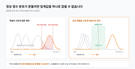
[Figure 3] The threshold-setting trade-off

Set the threshold low, and variants whose score distributions sit high produce normal samples flagged as anomalies; set it high, and fine defects on variants whose distributions sit low get missed. So in the field, thresholds end up being set per variant — and at that moment, the explosion of management points from Part 1 replays itself. Hundreds of variants mean hundreds of thresholds to manage.

So we add one more stage to the training pipeline. After training, we pass the normal data through the model again, pick out the normal samples with unusually high scores, and retrain with their weight increased — a process of finding and filling the poorly learned regions. This narrows the normal-score distributions and reduces the positional gaps between variants, allowing multiple variants to run on a single threshold. This, far more than a few points of AUROC, determines how hard a system actually is to deploy.

What remains

An unsupervised model only tells you that something deviates from normal. It cannot tell whether that is a crack, a foreign particle, or a dent. This limitation leads to two practical problems: you cannot produce defect-type trend reports, and you cannot automatically decide whether a part should be reworked. On lines where rework versus scrap depends on the defect type, a person ends up looking again.

Yet going back to supervised learning revives the fourth problem from Part 1 — defects the model never learned get classified as normal. In the next post, we cover the architecture that puts both approaches into a single system.

[AI Inspection: Challenges in the Field] Series

Part 1. Starting AI Inspection Without Defective Products
Part 3. Why AIVEX Combines Supervised and Unsupervised Learning in a Single Model
Part 4. How We Processed Thousands of Product Variants with a Single Model
Part 5. What to Consider When Generating Defect Data for Model Training
Part 6. The Problem of Manually Aligning the Optical System Whenever the Product Variant Changes