[AI Inspection: Challenges in the Field (4)] Processing Thousands of Product Variants with a Single Model

In Part 1, we named the problem of models multiplying with every product variant as the fifth wall. This post is the story of consolidating them into one.

The direction itself is an old idea. Learning a shared representation once at scale and stacking individual tasks on top is a configuration that has taken hold across many fields. Bring it into inspection as-is, however, and it does not work well. This was never a problem that scaling up the backbone could solve.

If the data has to be cleaned before it goes in, the labeling effort remains as-is and the deployment timeline does not shrink. If one deployment shakes thousands of variants at once, operation becomes impossible. If the model cannot keep up with line speed, it is unusable regardless of accuracy. We will take these in order.

You cannot use a public backbone as-is

Let's start with what does not work.

First, the target is different. General vision models are trained to distinguish different objects from one another. Manufacturing inspection is the opposite: finding differences tens of micrometers in size between two nearly identical images. The background is a repeating pattern, defects are low-contrast, and the boundary between normal variation and defect is blurry. The representation demanded of the model is different.

Second, the resolution assumption breaks. Public backbones generally assume inputs a few hundred pixels across. Shrink an inspection image to that size, and the fine defects you are looking for are the first thing to disappear. The same constraint from Part 2 — that patch size cannot be set arbitrarily — applies at the pre-training stage as well.

Third, the data assumption is different. Large-scale training recipes generally assume clean, balanced data. Field data, however, is long-tailed and mixed with noise. Have engineers clean it first, and that effort becomes the deployment timeline; put it in uncleaned, and the model collapses on rare classes.

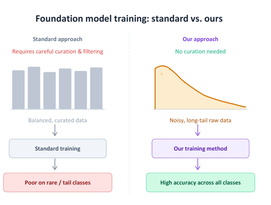
[Figure 1] Training that assumes clean data versus training that does not

We pre-train on data that accumulates without human hands

So we re-selected the pre-training material.

The criterion was a single one: it must be data that keeps accumulating without human hands touching it. Part 1 noted that defect data accumulates slowly — normal images are the opposite. They pile up simply by running the line, and they need no labels. These images, captured on the inspection line, become the pre-training material.

What diverged from here was the training method. As noted above, this data is not clean.

In pre-training, noise propagates differently

In supervised learning, one wrong label slightly shifts the decision boundary of that class. In pre-training, the stakes sit at a different level. What is being built here is not the judgment criterion for one variant but the representation every variant stacked on top will share. Once the representation space settles in the wrong place, every variant added afterward — however many — starts from there. Contamination that would have stayed confined to one variant under per-variant models spreads to the whole under a unified model.

That makes the decision to feed in uncleaned data a riskier choice at the pre-training stage. To take that risk, the model has to be able to filter contamination by itself during training.

The clue is in how the loss moves. As training progresses, the majority normal patterns converge first. Samples that entered by mistake, being inconsistent with the data around them, keep their loss high to the end. Using this difference — lowering the contribution of samples with abnormally high loss — weakens the pull that contaminated samples exert on the representation space.

The problem is that this criterion cannot be used as-is. Rare surfaces with only a few examples also keep their loss high to the end, because there is too little data for them to be sufficiently learned. Suppress all high-loss samples across the board, and rare patterns get erased along with the noise. The tail-versus-noise dilemma from Part 2 reappears at pre-training scale.

The clue for telling them apart is also the same as in Part 2. Noise has high loss and no mutual resemblance — its causes vary, so it scatters across the feature space. Rare patterns have high loss but resemble one another, having come from the same surface of the same variant. Look not at loss magnitude alone but at whether the sample has neighbors in the feature space, and what should be suppressed separates from what should be kept.

This carries the discrimination used for memory-bank condensation in Part 2 over into the loss weighting of training. The point of application differs, but the question asked is the same: is this sample rare by nature, or did it enter by mistake?

Rare patterns are shown often but learned gently

Loss design alone is not enough. If a sample never appears during training in the first place, no weighting scheme matters.

Sample the data uniformly, and common surfaces numbering in the tens of thousands occupy most of the training steps. A rare variant with only a few examples appears just a handful of times per epoch, and even those get buried under the gradients of common patterns. So we raise the appearance frequency of rare patterns.

But raise frequency alone, and you tip over to the other side. With only a few source images shown often, the model memorizes those few. It is the same trap noted in Part 1 — oversampling rare classes only increases overfitting.

So we separated the two: raise the appearance frequency, but lower how much each appearance moves the parameters. Rare patterns get reflected a little at a time across many appearances; common patterns appear less often but are reflected normally each time. The result is a model that knows rare surfaces exist without memorizing those specific images.

The goal is simple: not "clean up the data and we will train on it" but "give it to us as it is." Labeling and preprocessing effort is deployment time, and deployment time is cost.

One more thing worth settling here. We are often asked whether this means pooling multiple customers' data into one model. It does not. Pre-training is performed only on data cleared for transfer and on public data; each customer's data is reflected only in that customer's own layers, within their own site. The same principle holds in air-gapped configurations.

Variant differences are absorbed by thin layers

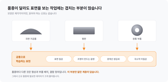
[Figure 2] Shared feature representation across variants

The texture of metal, the shading that lighting creates, the way edges look, the local incongruity when a foreign particle sits on a surface — these do not differ much whether the part is a curved machined piece, a flat panel, or a cylindrical component. What differs per variant is the geometry, the component layout, and the definition of what counts as a defect.

So the shared part up front is handled by the pre-trained representation, and only the per-variant differences are carried by thin layers stacked on top. The word thin is the important condition here. Fully fine-tune down to the backbone for every new variant, and you end up with as many weight sets as variants — the point of unification disappears. On top of that, every time a new variant is trained, the performance of previous variants degrades. Freeze the backbone, and the parameter increase per variant is held to a minimum, with no effect on existing variants.

The procedure for onboarding a new variant becomes simple as well. What the engineer does ends at securing normal images for that variant and training only the thin layer. There is no need to collect defect data from the start. A tire full-surface appearance inspection line we operate handles thousands of specifications on a single model this way, and the data required for training dropped to a level tens of times smaller than the per-variant approach — because almost nothing is left for each variant to learn from scratch.

Here the question arrives from the opposite direction: doesn't merging thousands of variants into one mean giving up per-variant optimization?

The result was the opposite. A per-variant model sees only that variant's data, so the less data a variant has, the poorer its training. A unified model looks at each variant having already learned the surfaces and defects seen on other variants. A defect shape appearing for the first time on one variant has often already been seen on another, and generalization benefits accordingly. On the few variants with abundant data, a dedicated model may edge ahead slightly — but averaged across all variants, the unified model came out ahead. And in inspection, the trouble usually comes from the data-poor side.

Large models are slow

Inspection lines have a takt time. Within the interval one product takes to pass, imaging, inference, and judgment must all finish. This is why many sites have chosen either a light model at the cost of precision, or precision at the cost of line speed.

The first thing we looked at was not compute but memory. Profile it, and what consumes time on the GPU is often memory access rather than the computation itself. Attention-family operations in particular spend most of their time shuttling intermediate results out of fast memory and back in. So we rebuilt the bottleneck layers on top of an implementation that maximizes fast-memory utilization.

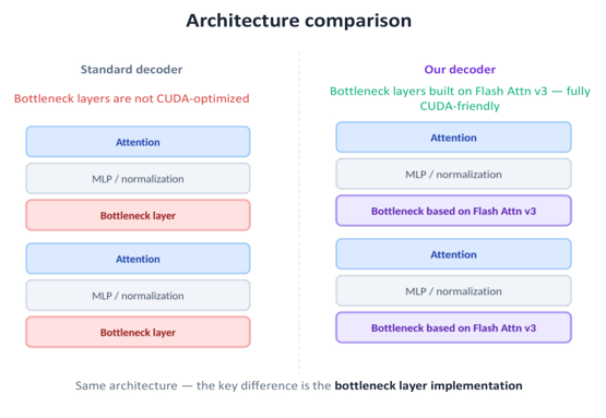
[Figure 3] Decoder structure with only the bottleneck-layer implementation swapped

The overall architecture is identical; only the bottleneck-layer implementation changed. On top of this, instead of general-purpose libraries, we attached our own decoder that issues instructions directly to the accelerator.

The second is quantization — which, in inspection, is hard to apply as-is. Fine defects have low contrast, so lowering precision smears the difference against the background first. So rather than lowering all layers uniformly, we measure how much detection performance drops when each layer's precision is reduced, and leave the high-loss sections at original precision.

The third lies outside the model. Optimize inference alone while leaving image decoding and resizing on the CPU, and that becomes the new bottleneck. We have in fact seen a case where model inference was cut in half yet total takt barely moved. Treating everything from imaging to judgment as one pipeline and measuring the time share of each stage gets you to real improvement faster.

Put together, this yields inference up to 3x faster than a model of the same parameter scale. On the tire line, over 100 high-resolution images per product are processed within a 30-second takt; on a precision-parts line, sub-1-second takt is maintained. A side effect is a reduction in the number of inference GPU servers — and the more inspection lines a factory has, the more directly that difference shows up in the initial investment.

What remains

By this point, the many-variants situation is largely settled. Normal images for a new variant accumulate just by running the line, and training the thin layer on them is all it takes.

The defect side, however, remains as it was. A foundation model reduces the data requirement, but the situation of having only a handful of defect samples to train on is still with us.

The next post takes that on.

[AI Inspection: Challenges in the Field] Series

Part 1. Starting AI Inspection Without Defective Products
Part 2. What Actually Goes Wrong When Detecting Anomalies Using Only Normal Samples
Part 3. Why AIVEX Combines Supervised and Unsupervised Learning in a Single Model
Part 5. What to Consider When Generating Defect Data for Model Training
Part 6. The Problem of Manually Aligning the Optical System Whenever the Product Variant Changes